A logical interpretation of the function subtyping rule

We discussed the subtyping rule for function type in this post. In short, a function type is contravariant in the argument types and covariant in the result type. Several days ago, I happened to notice that the Monotonicity Theorem for implication (see p.70 in [1]) looks very similar to the aforementioned subtyping rule in form. Given propositions $p,p',q,q'$ such that $p'\Rightarrow p$ and $q'\Rightarrow q$, the theorem asserts $$p'\vee q' \Rightarrow p \vee q.$$ Besides, it is immediate to see that $p \vee q \equiv \neg q \Rightarrow p$ and $q' \Rightarrow q \equiv \neg q \Rightarrow \neg q'$, assuming the law of double negation. Now, by writing $p$, $p'$, $\neg q$ and $\neg q'$ as $P$, $P'$, $Q$ and $Q'$, respectively, we obtain \begin{equation} (Q' \Rightarrow P') \Rightarrow (Q \Rightarrow P) \label{subtyping} \end{equation} given that $P'\Rightarrow P$ and $Q\Rightarrow Q'$.

The connection between the above fact and the subtyping rule of function types can be established by treating the implication connective "$\Rightarrow$" as both a function-type constructor and a subtype-of relation. Indeed, if Apple is a subtype of Fruit then being an Apple implies being a Fruit. It is thus reasonable to use "Apple $\Rightarrow$ Fruit" to express the subtyping relation between Apple and Fruit. In view of this, the logical entailment in \eqref{subtyping} leads us to the following statement for function types: If $P'$ is a subtype of $P$ (i.e. $P' \Rightarrow P$) and $Q$ is a subtype of $Q'$ (i.e. $Q \Rightarrow Q'$), then function type $Q' \Rightarrow P'$ is a subtype of function type $Q \Rightarrow P$ (i.e. $(Q' \Rightarrow P') \Rightarrow (Q \Rightarrow P)$). In other words, a function type is contravariant in the argument types and covariant in the result type.

Reference

1. Gries, David, and Fred B. Schneider. "A logical approach to discrete math." Springer, 1993.

A note on the strong law of large numbers

I.i.d. r.v.s with zero mean

Consider a sequence of i.i.d. random variables $X_0, X_1, ....$ When the variance is finite, the sequence $S_0, S_1, ...$ of partial sums is expected to have a faster rate of convergence than the rate guaranteed by the Strong Law of Large Numbers (SLLN). In fact, we have the following theorem:

Theorem 2.5.1. If $Var(X_n)<\infty$ and $E[X_n]=0$, then $\lim_{n\rightarrow\infty} (S_n/n^p)=0$ a.s. for all $p>\frac{1}{2}$.

This theorem can be proven using criteria of convergent series and the Borel-Cantelli lemma.

Indep. r.v.s with zero mean and finite sum of variance

It is possible to use a denominator with a slower growing rate than $n_p$. However, we will need a stronger assumption for the variances to ensure convergence without a divergent denominator.

Theorem 2.5.3. If $\sum_{n\ge1} Var(X_n)<\infty$ and $E[X_n]=0$, then $S_n$ converges a.s.

For sequences with $E[X_n]\neq0$, we can consider $Y_n=X_n-E[X_n]$ instead of $X_n$. Note that $Var(Y_n)=Var(X_n)$ and $E[Y_n]=0$. It then follows from the theorem that $\sum Y_n=\sum (X_n-E[X_n])$ converges a.s.

The ultimate characterisation of independent r.v.s with convergent partial sums is given by Kolmogorov.

Theorem 2.5.4. (Kolmogorov's Three-Series Theorem) Given independent $\{X_n\}$ and $a>0$, define $Y_n=X_n\cdot 1\{|X_n|\le A\}$. Then $S_n$ converges a.s. iff the followings all hold:
(i) $\sum \Pr\{|X_n|>A\}<\infty$, (ii) $\sum E[Y_n]<\infty$, and (iii) $\sum Var(Y_n)<\infty$.

Observe that $\sum_{n\ge1}Y_n<\infty$ a.s by the 2nd condition. Also, putting the 3rd condition and Theorem 2.5.3 together leads to the fact that $\sum_{n\ge1}(Y_n-E[Y_n])$ converges a.s. Finally, $\Pr\{X_n=Y_n$ for $n$ large$\}=1$ by the 1st condition and the Borel-Cantelli lemma. Hence, we see that $\sum_{n\ge1}X_n$ converges a.s. We need the Lindeberg-Feller theorem to prove the other direction.

Convergence of sequence is linked to the SLLN by the following theorem.

Theorem 2.5.5. (Kronecker's Lemma) If $a_n\nearrow\infty$ and $\sum_{n\ge1}b_n/a_n$ converges, then $\sum_{n\ge1}^N b_n/a_N \rightarrow 0$ as $N\rightarrow\infty$.

I.i.d. r.v.s with finite mean

The SLLN follows by Kolmogorov's Three-Series Theorem and Kronecker's Lemma.

Theorem 2.5.6. (SLLN) If $E[X_n]=\mu$, then $S_n/n=\mu$ a.s.

Faster rate of convergence

We can prove a faster rate of convergence under stronger assumptions.

Theorem 2.5.7. Suppose that $\{X_n\}$ are i.i.d., $E[X_n]=0$ and $\sigma^2=E[X_n^2]$, then for all $\epsilon>0$, $$\lim\frac{S_n}{\sqrt n (\log n)^{1/2+\epsilon}}=0\quad a.s.$$The most exact estimate is obtained from Kolmogorov's test (Theorem 8.11.3): $$\lim\frac{S_n}{\sqrt n (\log \log n)^{1/2}}=\sigma\sqrt 2\quad a.s.$$
Theorem 2.5.8. Suppose that $\{X_n\}$ are i.i.d., $E[X_n]=0$ and $E[X^p]<\infty$ for $1<p<2$. Then $\lim S_n/n^{1/p}=0$ a.s.

Examples

Example 2.5.3. Suppose $\{X_n\}$ is indep. and $\Pr\{X_n=\pm n^{-p}\}=1/2$. Then $p>1/2$ iff $S_n$ converges a.s. (Hint: use Theorem 2.5.4 and let $A=1$)

References

Rick Durrett. Probability: Theory and Examples. Edition. 4.1.

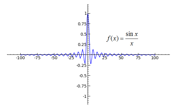
A note on the Riemann integral of sin(x)/x

In this post, we will prove the famous result that \[ \int_{0}^{\infty}\frac{\sin x}{x}dx=\frac{\pi}{2}. \] We first fix some $0<a<\infty$ and consider $e^{-xy}\sin x$. We shall show that $e^{-xy}\sin x$ is integrable on $0<x< a$ and $y>0$. As $\left|\sin x\right|\le1$, one may instead try to prove the integrability of $e^{-xy}$ for this purpose. Unfortunately, the attempt would fail since \[ \int_{0}^{a}\int_{0}^{\infty}e^{-xy}\,dy\,dx=\int_{0}^{a}\frac{1}{x}dx=\infty \] diverges. Bounding $e^{-xy}\sin x$ with $e^{-xy}$ turns out to be too rough near $x=0$, because $1/x\rightarrow\infty$ but $\sin x/x\rightarrow1$ when $x\searrow0$. We therefore need to use a tighter bound near $x=0$ to make the integral finite. Observe that, since $\sin x/x\rightarrow1$, given $\varepsilon>0$ there exists $\delta>0$ such that $\left|\sin x/x-1\right|< \varepsilon$ for $0< x< \delta$. Hence, \begin{eqnarray*} \int_{0}^{a}\int_{0}^{\infty}e^{-xy}\sin x\,dy\,dx & = & \int_{0}^{\delta}\int_{0}^{\infty}e^{-xy}\sin x\,dy\,dx+\int_{\delta}^{a}\int_{0}^{\infty}e^{-xy}\sin x\,dy\,dx\\ & \le & \int_{0}^{\delta}\frac{\sin x}{x}dx+\int_{\delta}^{a}\frac{1}{x}dx\\ & \le & \left(1+\varepsilon\right)\delta+\ln a-\ln\delta < \infty. \end{eqnarray*} Similarly, \[\int_{0}^{a}\int_{0}^{\infty}e^{-xy}\sin x\,dy\,dx \ge \left(1-\varepsilon\right)\delta-\ln a+\ln\delta > -\infty. \] It follows that the integral indeed exists. Now we can perform the double integral in two orders to obtain \[ \int_{0}^{a}\left(\int_{0}^{\infty}e^{-xy}\, dy \right)\sin x\, dx=\int_{0}^{a}\frac{\sin x}{x}dx \] and \begin{eqnarray*} \int_{0}^{\infty}\left(\int_{0}^{a}e^{-xy}\sin x \, dx \right) dy & = & \int_{0}^{\infty}\left(\dfrac{1}{y^{2}+1}-\dfrac{\left( \cos a + y\,\sin a \right)e^{-ay}}{y^{2}+1}\right) dy \\ & = & \frac{\pi}{2}-\cos a\int_{0}^{\infty}\frac{e^{-ay}}{1+y^{2}}dy-\sin a\int_{0}^{\infty}\frac{y\,e^{-ay}}{1+y^{2}} dy \end{eqnarray*} Hence, \begin{eqnarray*} \left|\int_{0}^{a}\frac{\sin x}{x}dx-\frac{\pi}{2}\right| & = & \cos a\int_{0}^{\infty}\frac{e^{-ay}}{1+y^{2}}dy+\sin a\int_{0}^{\infty}\frac{y\,e^{-ay}}{1+y^{2}}dy\\ & \le & \int_{0}^{\infty}\left(1+y\right)e^{-ay}\, dy\\ & = & a^{-2}+a^{-1}. \end{eqnarray*} By taking $a\rightarrow\infty$ we obtain the desired result.

You can find different proofs of the same result here. Besides, this thread shows why $\sin{x}/x$ is Riemann integrable but not Lebesgue integrable on $(0,\infty)$.

An algebraic method for a graph decomposition problem

Let $K_{n}$ denote an $n$-clique and $K_{n,m}$ denote a complete bipartite graph. We are interested in the least number $m$, denoted as $m(n)$, such that $K_{n}$ can be edge-decomposed into $m$ complete bipartite graphs. Observe that $m(1)=0$, $m(2)=1$, $m(3)=2$, $m(4)=3$, etc. It is not difficult to deduce $m(n)\le n-1$ after some case studies, since we can obtain a decomposition of $K_{n+1}$ by adding $K_{1,n}$ to a decomposition of $K_{n}$, which implies $m(n+1)\le m(n)+1$. The nontrivial part lies in the reverse direction: how can we prove a strict lowerbound for $m(n)$? If we want to establish the lowerbound by analyzing the graphs directly, we have to show for all $K_n$ that there is no better decomposition than the one we offer, and this is far from an easy job.

R.$~$Graham proposed a very clever method to establish $m(n)\ge n-1$ based on elementary knowledge from linear algebra. He used $n$ variables $x_{1},...,x_{n}$ to represent the $n$ vertices $v_{1},...,v_{n}$ of $K_{n}$. An edge $\overline{v_{i}v_{j}}$ is selected iff $x_{i},x_{j}$ are both nonzero. The key observation is: if $(A_{1},B_{1}),...,(A_{m},B_{m})$ is a decomposition of $K_{n}$ into complete bipartite graphs, then the equation \[ \sum_{1\le i < j\le n}x_{i}x_{j}=\sum_{k=1}^{m}\sum_{x\in A_{k}}\sum_{y\in B_{k}}xy=\sum_{k=1}^{m}\left(\sum_{x\in A_{k}}x\right)\left(\sum_{y\in B_{k}}y\right) \] must holds for any assignment of $x_{1},...,x_{m}$. (An equation like this is called a double counting in the buzzwords of Combinatorics.)

With the observation in mind, he considered the following homogeneous system of linear equations: \[ \begin{cases} \sum_{i=1}^{n}x_{i}=0,\\ \sum_{x\in A_{k}}x=0, & k=1,...,m \end{cases} \] Now suppose that $m < n-1$. The system then has $n$ unknowns and $m+1 < n$ equations. This implies that the system has an infinitely number of solutions. In particular, there exists a nontrivial assignment for $x_{1},...,x_{n}$ such that \[ 2\cdot\sum_{1\le i < j\le n}x_{i}x_{j}=\left(\sum_{i=1}^{n}x_{i}\right)^{2}- \sum_{i=1}^{n}x_{i}^{2}=-\sum_{i=1}^{n}x_{i}^{2}=0, \] which is impossible since the last equality enforces $x_{1}=...=x_{n}=0$. It follows that $m(n)\ge n-1$ by contradiction. Hence, we can conclude $m(n)=n-1$.

A note on expectation transformer semantics

An expectation is a function that maps program states to either a nonnegative real value, or a non-negative real-valued expression over state variables. When the program contains randomized operations, an expectation here is in fact a nonnegative random variable over the distribution induced by the reachability probability of program states. An expectation is called a post-expectation when it is to be evaluated in on final states. An expectation is called a pre-expectation if it is to be evaluated on initial states.

Intuitively, we may regard a post-expectation as a random variable representing nonnegative "rewards" of final states. One can examine the program beforehand to estimate for each initial state the expected rewards when the program runs repeatedly from there. This estimate, called the weakest pre-expectation, is a nonnegative function that maps an initial state to the expected reward over the final states starting from that state. In other words, a weakest pre-expectation evaluates to the expected value of the post-expectation over the distribution of final states produced by program executions.

Given a probabilistic program $prog$ and a post-expectation $postE$ over final states, we use $wp(prog,postE)$ to denote the weakest pre-expectation of $prog$ with respect to $postE$. As a function over state variables, $wp(prog,postE)$ maps an initial state of $prog$ to the expected value of $postE$ in the final distribution reached via executions of $prog$. In particular, $wp(prog,1)$ maps an initial state to the probability that the program will terminate from that state, and $wp(prog,[pred])$ is the probability that the program will terminate in a state satisfying predicate $pred$. (Here we use square brackets $[\cdot]$ to denote an indicator function, so that given a predicate $pred$, $[pred]$ evaluates to 1 on states satisfying $pred$ and evaluates to 0 otherwise.)

Expectations are quantitative analogue to predicates in the predicate transformer semantics; they yield expectation transformer semantics of probabilistic programs. An expectation transformer is a total function between two expectations on the states of a program. The expectation transformer $wp(prog,postE)$ gives the least expected value of $postE$ over the distribution produced by the executions of $prog$. The annotation $\langle {preE} \rangle\; prog\;\langle {postE} \rangle$ holds for total correctness if and only if \begin{equation} preE\le wp(prog,postE),\label{eq:pre-wp-post} \end{equation} where $\le$ is interpreted in a point-wise manner. In other words, $preE$ gives in each initial state a lower bound for the expected value of $postE$ on final states when $prog$ starts from that initial state.

In the special case when expectations $preE$ and $postE$ are given by $[pre]$ and $[post]$, respectively, where $pre$ and $post$ are predicates, annotation $\langle {preE} \rangle\; prog\;\langle {postE} \rangle$ is just the embedded form of a standard Hoare-triple specification $\{pre\}\; prog\;\{post\}$, i.e., we can assume the truth of $post$ after the execution of $prog$, provided $pre$ holds in the initial state. More precisely, we have \[ [pre]\le wp(prog,[post])\quad\mbox{iff}\quad pre\Rightarrow wp(prog,post). \]In this view, inequality between expectations in expectation transformer semantics can be seen as a generalization of implication between predicates in predicate transformer semantics.

Reference

McIver, Annabelle, and Charles Carroll Morgan. "Abstraction, refinement and proof for probabilistic systems." Springer, 2006.

A note on predicate transformers and loop invariants

For standard programs, the computational model of execution supports a "logical" view—given a set of final states, we can examine the program to determine the largest set of initial states from which execution of the program is guaranteed to reach the final states. The sets of states are characterized by logical formula called predicates, and the program is being regarded as a predicate transformer, i.e., a total function that maps one predicate to another. We give some important terminology before we proceed:

• An assertion is a predicate placed in a program to assert that it holds at that point
• A precondition is an assertion placed before a program segment
• A postcondition is an assertion placed after a program segment
• A formula in form $\{precond\} \; program \; \{postcond\}$ is called a Hoare triple
• A Hoare triple is valid iff whenever the precondition holds, the postcondition holds after the execution of the program segment terminates
• A loop invariant is an assertion supposed to be true before and after each iteration of a loop

The following example puts all ingredients together:

// Precondition: (x=0 and y=0 and n≥0)
while (y<n) { 
    // Loop invariant: 2*x = y*(y-1)
    x+=y; y++; 
}
// Postcondition: 2*x = n*(n-1)

Observe that $\{x=0 \wedge y=0 \wedge n\ge0\}$ while(y<n){x+=y;y++;} $\{2x=n(n-1)\}$ is a valid Hoare triple and $2x = y(y-1)$ is an invariant for the while loop.

Predicate transformer semantics provide an effective algorithm to verify a Hoare triple by reducing the verification problem to the problem of proving logical entailment: Given a Hoare triple $\{pre\} \; prog \; \{post\}$, we first compute the weakest precondition of executing $prog$ starting from $post$, and then check that it entails $pre$. This amounts to proving that $$pre \Rightarrow wp(prog, post).$$When $prog$ doesn't contain a loop, the weakest precondition is simply given by syntactic rules. However, the presence of loops may pose a problem because the precondition is given in terms of a least fixed point. Besides, a separate proof is required to establish that the loops terminate from their initial state. Formally, if $G$ is a predicate and $body$ is a loop-free program segment, then \begin{equation} wp({\rm while}(G)\{body\}, post) = \mu X.((G\Rightarrow wp(body, X)) \wedge (\neg G\Rightarrow post)),\label{loop-wp} \end{equation} where $\mu$ is the least fixed point operator w.r.t. logic implication. Given that the loop terminates and the least fixed point exists, the construction of the weakest precondition can be sketched in set theory as follows. Let $\Sigma$ denote the state space. We define a family $\{A_k:k\ge0\}$ of subsets of $\Sigma$ by induction over $k$: \begin{array}{rcl} A_0 & = & \emptyset \\ A_{k+1} & = & \left\{\ y \in \Sigma: ((G \Rightarrow wp(body, x \in A_k)) \wedge (\neg G \Rightarrow post))[x \leftarrow y]\ \right\} \\ \end{array} Informally, $A_k$ represents the set of initial states that makes the postcondition $post$ satisfied after less than $k$ iterations of the loop. We can then define the weakest precondition in \eqref{loop-wp} as a first-order predicate $\exists k. x \in A_k$.

While an abstract construction as above is elegant, it can not be handled efficiently by theorem provers in practice. Fortunately, using special assertions called loop invariants we may by and large avoid the need of calculating fixed points. Suppose that we want to verify \begin{equation} pre \Rightarrow wp({\rm while} (G) \{body\}, post).\label{loop-hoare} \end{equation} Instead of calculating the least fixed point of the loop directly, we may divide the problem into simpler subtasks:

1. Find an assertion $I$ such that $pre \Rightarrow I$ and $I\wedge\neg G \Rightarrow post$.
2. Show that $I$ is an invariant: $I\wedge G \Rightarrow wp(body, I)$.
3. Show that $I$ is sound: $I \Rightarrow wp({\rm while}(G)\{body\}, I\wedge\neg G)$.

The first task ensures that the existence of $I$ establishes the desired relation between $pre$ and $post$. The second task considers a single iteration of the loop body and ensures that the execution of the loop preserves the validity of $I$. Note that it is easy to compute $wp(body, I)$ because $body$ is loop-free by assumption. In the third task, we check the soundness property such that every execution of the loop from a state satisfying the invariant can only terminate in a state that also satisfies the invariant and violates the guard $G$. It is still an open problem in the literature to give a necessary and sufficient condition for the soundness. On the other hand, soundness property can be established if one can show, e.g., by using a loop variant, that the loop terminates when it started from a state satisfying $I$.

With invariant $I$, the relation between $pre$ and $post$ in \eqref{loop-hoare} is established as $$pre \Rightarrow I \Rightarrow wp({\rm while}(G)\{body\}, I\wedge\neg G)\quad {\rm and }\quad I\wedge\neg G \Rightarrow post.$$ Checking correctness for code without loops turns out be easy in practice. Hence, the crucial point in verifying a Hoare triple is to discover the necessary loop invariants for each loop in the program.

References

Gries, David. "The science of programming." Vol. 1981. Heidelberg: Springer, 1981.