This is ericpony's blog

Friday, January 23, 2015

Deterministic aggregate semantics in Scala and Spark

The aggregate function in Scala has method signature as follows:
def aggregate[A](z: => A)(seqOp: (A, B) => A, combOp: (A, A) => A): A
The semantics of aggregate depend on the collection upon which it is invoked. When aggregate is invoked on a sequential traversable collection such as a List, it fallbacks to foldLeft and ignores the provided compOp. In this case, aggregate behaves just like the ordinary fold in typical functional programming languages such as Lisp and ML. When aggregate is invoked on a parallel traversable collection, however, it performs a two-stage aggregation over the data elements in parallel. In Scala, a parallel collection can be splitted into partitions and distributed over several cores or nodes. Invoking aggregate on a parallel collection reduces a value for the collection by first folding each partition separately using seqOp, and then merging the results one by one using combOp.

Note that the Scala API document doesn't specify the way in which the collection is partitioned, as well as the order in which the intermediate results are merged. Hence, if a programmer hopes to obtain the same output whenever aggregate is invoked on the same parallel collection, he has to make sure himself that seqOp is associative and combOp is both associative and commutative.

Aggregate v.s fold

The fold function in Scala has method signature as follows:
def fold[A1 >: A](z: A1)(combOp: (A1, A1) => A1): A1
One can observe two differences between the signatures of fold and aggregate: 1) fold only needs one operator, while aggregate needs two; 2) fold requires the result type to be a supertype of the element type, while aggregate doesn't. Note that both methods fallback to foldLeft when they are invoked on a sequential collection. One may notice that Scala's aggregate is in effect the ordinary FP fold
fold :  (A → B → A) → A → ([B] → A)
and Scala's fold is just a special form of its aggregate. The idea behind this design is to allow for parallel FP fold. In Scala, fold and aggregate are both done in two stages, namely folding and combining. For fold, the same operator is used for folding and combining, and this requires the supertype relationship between the element and the result type. Without the supertype relationship, it will take two operators to fold and combine, and this is why Scala provides aggregate that takes two operators as arguments.

Aggregate in Spark

Spark implements its own aggregate operations for RDD. One can observe from the source code of Spark that the intermediate results of aggregate are always iterated and merged in a fixed order (see the Java, Python and Scala implementations for details). Hence, we don't have to use commutative combOp to obtain deterministic results from aggregate, given that at least one of the following conditions holds:
(i) there doesn't exist an empty partition in any partitioning of the collection, or
(ii) z is an identity of combOp, i.e., for all a of type A, combOp(z,a) = combOp(a,z) = a.
Note that this observation is not assured by the official Spark API document and is thus not guaranteed to hold in the future versions of Spark. However, it is still useful if we want to model the behaviours of a Spark program formally.

Below, we shall try to formalize Spark's implementation of aggregate. While Scala is an impure functional language, we only consider pure functions here for simplicity. Let $R(L,m)$ denote an RDD object obtained from partitioning a list $L \in \mathbb{D}^*$ into $m \ge 1$ sub-lists. Suppose that we have fixed an element $zero \in \mathbb{E}$, as well as operators $seq:{\mathbb{E} \times \mathbb{D} \to \mathbb{E}}$ and $comb:{\mathbb{E} \times \mathbb{E} \to \mathbb{E}}$. An invocation of aggregate is said to be deterministic with respect to $zero$, $seq$ and $comb$ if the output of $$R(L,\cdot).\textrm{aggregate}(zero)(seq,\ comb)$$ only depends on $L$. Define a function $\textrm{foldl}:({\mathbb{E} \times \mathbb{D} \to \mathbb{E}}) \times \mathbb{E} \times \mathbb{D}^* \to \mathbb{E}$ by \begin{eqnarray*} \textrm{foldl}(f,\ a,\ Nil) & = & a \\ \textrm{foldl}(f,\ a,\ b \!::\! bs) & = & \textrm{foldl}(f,\ f(a,b),\ bs), \end{eqnarray*} where $f\in {\mathbb{E} \times \mathbb{D} \to \mathbb{E}}$, $a \in \mathbb{E}$, $b \in \mathbb{D}$ and $bs \in \mathbb{D}^*$. Suppose that $1\le m \le |L|$ and $R(L,m)$ partitions $L$ into $\{L_1, \dots, L_m\}$ such that $L=L_1 \cdots L_m$. According to the source code of Spark, we can define the aggregate operation in Spark as \begin{eqnarray*} R(L,m).\textrm{aggregate}(zero)(seq,\ comb) = \textrm{foldl}(comb,\ zero,\ L'), \end{eqnarray*} where $L' \in \mathbb{E}^*$ is a list of length $m$ and $L'[i] = \textrm{foldl}(seq,\ zero,\ L_i)$ for $i=1,\dots,m$.

Note that the partitioning of $L$ is unspecified and may be non-deterministic. Hence, we have to use an associative $comb$ operator if we want to ensure that the result of aggregation is deterministic. Suppose that $comb$ is associative and at least one of conditions (i) and (ii) is satisfied. It turns out that the output of aggregate is deterministic with respect to $zero$, $seq$ and $comb$ if and only if for all lists $L_1$ and $L_2$, $$comb(zero,\ \textrm{foldl}(seq,\ zero,\ L_1L_2)) = comb(\textrm{foldl}(seq,\ zero,\ L_1),\ \textrm{foldl}(seq,\ zero,\ L_2)).$$ While the above condition is undecidable in general, it can be effectively checked for some classes of programs such as FSMs over finite alphabets.

Concluding remarks

Aggregate in Spark is the parallelized version of the conventional fold, which was already shown to be extremely useful in functional programming. It is therefore of practical interests to study the properties and behaviours of the aggregate function. In particular, it is interesting to establish and verify the conditions under which aggregate is deterministic with respect to the provided $zero$, $seq$ and $comb$. We may further investigate this problem in the coming posts.

Thursday, January 15, 2015

Emulating Hadoop in Spark

The map and reduce functions in MapReduce have the following general form:
Map: (K1, V1) → list(K2, V2)
Reduce: (K2, list(V2)) → list(K3, V3)
When a MapReduce program is executed, the Map function is applied in parallel to every pair in the input dataset. Each invocation of map produces a list of pairs. The execution framework then collects all pairs with the same key from all lists and groups them together, creating one group for each key. After that, the Reduce function is applied in parallel to each group, which in turn produces a collection of key-value pairs. In Hadoop's implementation of MapReduce, the values in the same group are sorted before they are sent to a reducer.

Despite the suggestive naming, map and reduce operations in Spark do not directly correspond to the functions of the same name in MapReduce. For example, Map and Reduce functions in MapReduce can return multiple key-value pairs. This feature can be implemented by the flatMap operation in Spark (and typical FP languages in general):
List(1, 2, 3).map(a => List(a))     // List(List(1), List(2), List(3))
List(1, 2, 3).flatMap(a => List(a)) // List(1, 2, 3)
One naive attempt to emulate Hadoop MapReduce (without combiners) in Spark is to use two flatMap operations for map and reduce, separated by a groupByKey and a sortByKey to perform shuffle and sort:
val input: RDD[(K1, V1)] = ...
val mapOutput: RDD[(K2, V2)] = input.flatMap(mapFn)
val shuffled: RDD[(K2, Iterable[V2])] = mapOutput.groupByKey().sortByKey()
val output: RDD[(K3, V3)] = shuffled.flatMap(reduceFn)
Here the key type K2 needs to inherit from Scala’s Ordering type to satisfy the signature of sortByKey. The above code is useful to demonstrate the relationship between Hadoop and Spark, but it should not be applied blindly in practice. For one thing, its semantics are slightly different from Hadoop's MapReduce, since sortByKey performs a total sort over all key-value pairs while Hadoop sorts within groups. This issue can be avoided by using repartitionAndSortWithinPartitions in Spark 1.2 to perform a partial sort:
val shuffled: RDD[(K2, Iterable[V2])] = mapOutput
    .groupByKey()
    .repartitionAndSortWithinPartitions(Partitioner.defaultPartitioner(mapOutput))
The improvement is unfortunately still not as efficient, since Spark uses two shuffles (one for the groupByKey and one for the sort) while MapReduce only uses one. It turns out one cannot precisely and efficiently capture the semantics of Hadoop's MapReduce in the current version of Spark.

Rather than trying to reproduce MapReduce in Spark, it is better to use only the operations that you actually need. For example, if you don’t need keys to be sorted, you can omit the sortByKey call to avoid sorting (which is impossible in regular Hadoop MapReduce). Similarly, groupByKey is too general in most cases. If shuffling is needed only for aggregating values, you should use reduceByKey, foldByKey, or aggregateByKey, which are more efficient than groupByKey since they exploit combiners in the map task. Finally, flatMap may not always be needed either. Instead, you can use map if there is always one return value, or use filter if there is zero or one.

Consult these two articles on Cloudera for details of translating Hadoop programs to efficient Spark programs: How-to: Translate from MapReduce to Apache Spark, part 1 and part 2.

Further readings

1. Jimmy Lin, Chris Dyer. Data-Intensive Text Processing with MapReduce.
2. Tom White. Hadoop: The Definitive Guide, 4th Edition.
3. Srinivasa, K.G., Muppalla, Anil K. Guide to High Performance Distributed Computing.

Monday, December 29, 2014

Basic dependent type theory ─ Part I

Computational trinitarianism. Proof Theory, Category Theory, and Type Theory, to a significant degree, can be regarded as fields that see the same subject from different points of view. They can be related via the follows:
TT ⇔ CT: category semantics; WTT corresponds to morphisms and categories.
PT ⇔ CT: category logic; an algebraic way of thinking about logic and proofs.
PT ⇔ TT: thinking propositions as types and WTT as proofs.
When you are learning a new idea in one field, it is helpful to transpose it to the other two fields and seek its correspondence there. See here and here for more details.
Judgements. We start with three kinds of categorical judgements:
$A\ type$   ─  $A$ is a type.
$a \in A$    ─  $a$ is a value of type $A.$
$a_1=a_2: A$ ─  $a_1$ and $a_2$ are "definitionally equivalent" values of type $A.$
A judgement in form of $x_1:A_1,...,x_n:A_n \models a(x_1,...,x_n):A$ is called a hypothetical judgement. One may regard such a judgement as a mapping from $A_1,...,A_n$ to $A.$ $a(x_1,...,x_n)$ is called an open term that might involve free variables $x_1,...,x_n.$ In practice, we often consider the open term parametrized at $x_1,...,x_n.$ A closed term of type $A$ can be determined categorically after the values of $x_1,...,x_n$ are plugged in.
Definitional equality is 1) an equivalence relation, 2) a congruence (see typing rules), and 3) respected by maps. That is, $$\frac{\Gamma, x:A \models b:B, \Gamma \models a_1\equiv a_2: A}{\Gamma \models [a_1/x]b \equiv [a_2/x]b : B}.$$The last feature is called the principle of functionality property. This property and its related concepts will play a central role later and in Homotopy type theory.
Definitional equality has its limits. For example, one cannot prove definitional equivalence between $0+1$ and $1+0$ even given all the arithmetic rules about natural numbers. Definitional equality corresponds to calculating by simplification. There however are equations (such as $0+1=1+0$) that you wish to hold cannot be reached that way. These equations need not just calculation but proof, and thus cannot hold definitionally.
Typing rules. We have the following kinds of rules to reason about types. Rules 1-5 come from Proof Theory and Rule 6 comes from Category Theory.
1. Formation rules: how to construct a type.
2. Introduction rules: how to create elements of a type.
3. Elimination rules: how to use elements of a type.
4. Congruence rules: how to interact with definitional equivalence.
5. Computation rules: how to do calculation with types
6. Uniquicity/Unisersality rules: characterize precisely types

Negative types. E.g., Unit, product, and function. Elimination-oriented. Uniquicity of product: $\Gamma \vdash \langle fst(c), snd(c) \rangle \equiv c : A\times B.$ Computation of function is substitution. Elimination of function is application. Extension of function can be written as $$\frac{\Gamma, x:A \vdash a_1(x)\equiv a_2(x):B}{\Gamma \vdash a_1\equiv a_2: A\rightarrow B}$$This means that functions are characterized by their input-output behaviors.
Positive types. E.g., Void and sum. Introduction-oriented. The Uniquicity property of positive types is problematic, and cannot be shown as for the negative types as directly. Elimination rule for the Void type:$$\frac{\Gamma\vdash a:\emptyset}{\Gamma\vdash abort(a): A}$$This means if you have a value of the Void type, you can abort the program with any type. Note that one can never build a term of type $A$ in this way since there is no closed term of type $\emptyset.$ One application of this rule is that if you are in a conditional branch, then one side of the conditional may be contradictory, and you can build an $abort$ element of type $A$ to make sure both elements for the condition have the same type.
Negative types vs. positive types. Approximately, the two types differ most noticeably in how they behave under elimination. Reasoning about a negative type has noting to do with its structure. For example, a product is characterized by its behaviors on $\texttt{fst}$ and $\texttt{snd}$ without caring about what it actually is. A product can be realized by an ordered pair or just a black box that computes the $\texttt{fst}$ and $\texttt{snd}$ components on demand. Also, there is no induction principle for negative types. For example, all you know about a function is that it is a lambda term. Thus you cannot induct on its structure via the typing rules. In contrast, the structure of a positive type is enforced in the theory. The elimination form of positive types work by case analysis─the actual element in a sum is extracted by $\texttt{case}$ in the process of inference. Thus it cannot be anything else after the inference.
A correspondence btw STT and IPT. $Unit$ is $true.$ $Void$ is $false.$ Sum is disjunction. Product is conjunction. Function is implication. $A\ type$ is $A\ prop.$ $\exists e: A$ is $A\ true.$ $\exists b.\, a:A \vdash b:B$ is $A\le B.$ Thus $A\le B$ means that there is a function transforming a proof for $A$ to a proof for $B.$ Note that $\le$ is a pre-order: that is, it is reflexive and transitive. We use $A\supset B$ to denote the largest element $x$ satisfying $A\wedge x \le B$, i.e., $C \wedge A \le B$ implies $C \le A \supset B.$ If an ordered structure satisfies 1) $\forall A: A\le \top$; 2) $\forall A: \bot \le A$; 3) $A\wedge B$ (meet) is a glb for $A,\,B$; 4) $A\vee B$ (join) is a sub for $A,\,B$; 5) $\wedge$ is distributive over $\vee$; 6) $A \supset B$ exists for every $A,B$, then it is called a Heyting pre-algebra. (It is called a pre-algebra because $\le$ is not anti-reflexive.)
Negations. $\neg\ A$ is defined as $A \supset \bot.$ Thus we can get a contradiction from a value of $A.$ The fact $A\le \neg\neg\ A$ follows directly by the properties of $\supset.$ Its converse $\neg\neg\ A \le A$ however doesn't hold in general (it takes quite some efforts to check this statement). Similarly, while $A \vee \neg\ A \le \top$ is trivial, $\top \le A \vee \neg\ A$ cannot be proved in general without knowing something about $A.$
By definition, $\neg A$ is the largest element inconsistent with $A.$ That is, $A\wedge\neg A \le \bot$ and $B\wedge\neg A \le \bot \implies B\le \neg A.$ The compliment $\overline{A}$ of $A$ is defined as the smallest element $B$ such that $\top\le A\vee\overline{A}.$ Hence $\top\le A\vee B$ implies $\overline{A}\le B.$ Note that i) $\neg A$ always exists while $\overline{A}$ does not; ii) it is reasonable to add the largest/smallest requirement to the definitions, for otherwise we can trivially choose $\neg\ A=\bot$ and $\overline{A}=\top$; iii) it is easy to check $\neg\ A \le \overline{A}$ (things in $\neg\ A$ are definitely not in $A$). The converse $\overline{A} \le \neg\ A$ however does not hold in general (the negation does not fill up the whole space).
A Boolean algebra is also called a complemented Heyting algebra in that $\overline{A}$ exists for every $A$, with i) $\top \le A\vee \neg\ A$ (which implies $A\vee \neg\ A=A\vee \overline{A}$), and ii) $\overline{\overline{A}} \le A$ (note that $A \le \overline{\overline{A}}$ follows by definition). Heyting pre-algebras generalize Boolean pre-algebras in the sense that a Heyting pre-algebra satisfying $1 \le A \vee \neg A$ (law of excluded middle), or equivalently $\neg\neg A \le A$ (law of double negation), is a Boolean pre-algebra.
Heyting algebras. An exponential $y^x$ is defined as $\overline{x}\vee y.$ A Heyting algebra can also be defined as a lattice with exponentials: $H$ is called a Heyting algebra if i) it has a preorder; ii) it has finite meets and joins, and iii) satisfies $y^x$ is the largest element $z$ such that $x \wedge z \le y.$
Exercise. Show that every Heyting algebra is distributive.
We give hints about proving $x \wedge (y \vee z) = (x \wedge y) \vee (x \wedge z).$ First, note that $z \wedge x \le y$ iff $z \le y^x.$ Hence, to prove direction $x \wedge (y \vee z) \le (x \wedge y) \vee (x \wedge z)$, it suffices to show $y \vee z \le ((x \wedge y) \vee (x \wedge z))^x$, which amounts to show that $u \le ((x \wedge y) \vee (x \wedge z))^x$ for $u=y, z.$ However, $u \le ((x \wedge y) \vee (x \wedge z))^x$ iff $u \wedge y \le (x \wedge y) \vee (x \wedge z).$ For $u=y, z$ this follows by definition. As to the other direction, note that $x \le y$ iff $\forall z.\,(y\le z$ $\implies x \le z).$ Hence, to prove $(x \wedge y) \vee (x \wedge z) \le x \wedge (y \vee z)$, it suffices to show that $(x \wedge y) \vee (x \wedge z) \le u$ implies $x \wedge (y \vee z) \le u$, which is equivalent to $y \vee z \le u^x.$ Note that $(x \wedge y) \vee (x \wedge z) \le u$ implies both $x \wedge y \le u$ and $x \wedge z \le u.$ Thus we have $y \le u^x$ and $z \le u^x$, that is, $y \vee z \le u^x.$
As an alternative, you can also use the completeness theorem for IPT. Completeness assures that anything that holds in every Heyting algebra must be provable in IPT, and vice versa. Since preorder is interpreted to entailment in IPT, you can transfer e.g., $x \wedge (y \vee z) \le (x \wedge y) \vee (x \wedge z)$ to $X \wedge (Y \vee Z)\ true \vdash (X \wedge Y) \vee (X \wedge Z)\ true$, and then reason about the logical connectives to do the proof. You can further add proof terms to obtain a FP problem $\Gamma, x: A \times (B + C) \vdash M: (A \times B) + (A \times C).$ Resolving this problem amounts to writing a program $M$ of type $(A \times B) + (A \times C)$, and it is not hard to see that $M = \texttt{case}(z.\,\texttt{inl}(\langle \texttt{fst}(x), z\rangle);\, z.\,\texttt{inr}(\langle \texttt{fst}(x), z\rangle))\ \texttt{snd}(x).$ It is sort of a cyclelogical matter for people to transfer problems around the trinitarian when they are doing proofs.

Wednesday, December 10, 2014

A logical interpretation of the function subtyping rule

We discussed the subtyping rule for function type in this post. In short, a function type is contravariant in the argument types and covariant in the result type. Several days ago, I happened to notice that the Monotonicity Theorem for implication (see p.70 in [1]) looks very similar to the aforementioned subtyping rule in form. Given propositions $p,p',q,q'$ such that $p'\Rightarrow p$ and $q'\Rightarrow q$, the theorem asserts $$p'\vee q' \Rightarrow p \vee q.$$ Besides, it is immediate to see that $p \vee q \equiv \neg q \Rightarrow p$ and $q' \Rightarrow q \equiv \neg q \Rightarrow \neg q'$, assuming the law of double negation. Now, by writing $p$, $p'$, $\neg q$ and $\neg q'$ as $P$, $P'$, $Q$ and $Q'$, respectively, we obtain \begin{equation} (Q' \Rightarrow P') \Rightarrow (Q \Rightarrow P) \label{subtyping} \end{equation} given that $P'\Rightarrow P$ and $Q\Rightarrow Q'$.

The connection between the above fact and the subtyping rule of function types can be established by treating the implication connective "$\Rightarrow$" as both a function-type constructor and a subtype-of relation. Indeed, if Apple is a subtype of Fruit then being an Apple implies being a Fruit. It is thus reasonable to use "Apple $\Rightarrow$ Fruit" to express the subtyping relation between Apple and Fruit. In view of this, the logical entailment in \eqref{subtyping} leads us to the following statement for function types: If $P'$ is a subtype of $P$ (i.e. $P' \Rightarrow P$) and $Q$ is a subtype of $Q'$ (i.e. $Q \Rightarrow Q'$), then function type $Q' \Rightarrow P'$ is a subtype of function type $Q \Rightarrow P$ (i.e. $(Q' \Rightarrow P') \Rightarrow (Q \Rightarrow P)$). In other words, a function type is contravariant in the argument types and covariant in the result type.

Reference

1. Gries, David, and Fred B. Schneider. "A logical approach to discrete math." Springer, 1993.

Tuesday, October 21, 2014

A note on the strong law of large numbers

I.i.d. r.v.s with zero mean

Consider a sequence of i.i.d. random variables $X_0, X_1, ....$ When the variance is finite, the sequence $S_0, S_1, ...$ of partial sums is expected to have a faster rate of convergence than the rate guaranteed by the Strong Law of Large Numbers (SLLN). In fact, we have the following theorem:

Theorem 2.5.1. If $Var(X_n)<\infty$ and $E[X_n]=0$, then $\lim_{n\rightarrow\infty} (S_n/n^p)=0$ a.s. for all $p>\frac{1}{2}$.

This theorem can be proven using criteria of convergent series and the Borel-Cantelli lemma.

Indep. r.v.s with zero mean and finite sum of variance

It is possible to use a denominator with a slower growing rate than $n_p$. However, we will need a stronger assumption for the variances to ensure convergence without a divergent denominator.

Theorem 2.5.3. If $\sum_{n\ge1} Var(X_n)<\infty$ and $E[X_n]=0$, then $S_n$ converges a.s.

For sequences with $E[X_n]\neq0$, we can consider $Y_n=X_n-E[X_n]$ instead of $X_n$. Note that $Var(Y_n)=Var(X_n)$ and $E[Y_n]=0$. It then follows from the theorem that $\sum Y_n=\sum (X_n-E[X_n])$ converges a.s.

The ultimate characterisation of independent r.v.s with convergent partial sums is given by Kolmogorov.

Theorem 2.5.4. (Kolmogorov's Three-Series Theorem) Given independent $\{X_n\}$ and $a>0$, define $Y_n=X_n\cdot 1\{|X_n|\le A\}$. Then $S_n$ converges a.s. iff the followings all hold:
(i) $\sum \Pr\{|X_n|>A\}<\infty$, (ii) $\sum E[Y_n]<\infty$, and (iii) $\sum Var(Y_n)<\infty$.

Observe that $\sum_{n\ge1}Y_n<\infty$ a.s by the 2nd condition. Also, putting the 3rd condition and Theorem 2.5.3 together leads to the fact that $\sum_{n\ge1}(Y_n-E[Y_n])$ converges a.s. Finally, $\Pr\{X_n=Y_n$ for $n$ large$\}=1$ by the 1st condition and the Borel-Cantelli lemma. Hence, we see that $\sum_{n\ge1}X_n$ converges a.s. We need the Lindeberg-Feller theorem to prove the other direction.

Convergence of sequence is linked to the SLLN by the following theorem.

Theorem 2.5.5. (Kronecker's Lemma) If $a_n\nearrow\infty$ and $\sum_{n\ge1}b_n/a_n$ converges, then $\sum_{n\ge1}^N b_n/a_N \rightarrow 0$ as $N\rightarrow\infty$.

I.i.d. r.v.s with finite mean

The SLLN follows by Kolmogorov's Three-Series Theorem and Kronecker's Lemma.

Theorem 2.5.6. (SLLNIf $E[X_n]=\mu$, then $S_n/n=\mu$ a.s.

Faster rate of convergence

We can prove a faster rate of convergence under stronger assumptions.

Theorem 2.5.7. Suppose that $\{X_n\}$ are i.i.d., $E[X_n]=0$ and $\sigma^2=E[X_n^2]$, then for all $\epsilon>0$, $$\lim\frac{S_n}{\sqrt n (\log n)^{1/2+\epsilon}}=0\quad a.s.$$The most exact estimate is obtained from Kolmogorov's test (Theorem 8.11.3): $$\lim\frac{S_n}{\sqrt n (\log \log n)^{1/2}}=\sigma\sqrt 2\quad a.s.$$
Theorem 2.5.8. Suppose that $\{X_n\}$ are i.i.d., $E[X_n]=0$ and $E[X^p]<\infty$ for $1<p<2$. Then $\lim S_n/n^{1/p}=0$ a.s.

Examples

Example 2.5.3. Suppose $\{X_n\}$ is indep. and $\Pr\{X_n=\pm n^{-p}\}=1/2$. Then $p>1/2$ iff $S_n$ converges a.s. (Hint: use Theorem 2.5.4 and let $A=1$)

References

Rick Durrett. Probability: Theory and Examples. Edition. 4.1.

Friday, October 10, 2014

A note on the Riemann integral of sin(x)/x

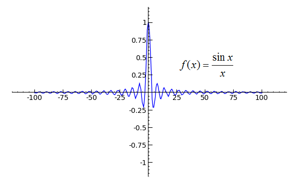
In this post, we will prove the famous result that \[ \int_{0}^{\infty}\frac{\sin x}{x}dx=\frac{\pi}{2}. \] We first fix some $0<a<\infty$ and consider $e^{-xy}\sin x$. We shall show that $e^{-xy}\sin x$ is integrable on $0<x< a$ and $y>0$. As $\left|\sin x\right|\le1$, one may instead try to prove the integrability of $e^{-xy}$ for this purpose. Unfortunately, the attempt would fail since \[ \int_{0}^{a}\int_{0}^{\infty}e^{-xy}\,dy\,dx=\int_{0}^{a}\frac{1}{x}dx=\infty \] diverges. Bounding $e^{-xy}\sin x$ with $e^{-xy}$ turns out to be too rough near $x=0$, because $1/x\rightarrow\infty$ but $\sin x/x\rightarrow1$ when $x\searrow0$. We therefore need to use a tighter bound near $x=0$ to make the integral finite. Observe that, since $\sin x/x\rightarrow1$, given $\varepsilon>0$ there exists $\delta>0$ such that $\left|\sin x/x-1\right|< \varepsilon$ for $0< x< \delta$. Hence, \begin{eqnarray*} \int_{0}^{a}\int_{0}^{\infty}e^{-xy}\sin x\,dy\,dx & = & \int_{0}^{\delta}\int_{0}^{\infty}e^{-xy}\sin x\,dy\,dx+\int_{\delta}^{a}\int_{0}^{\infty}e^{-xy}\sin x\,dy\,dx\\ & \le & \int_{0}^{\delta}\frac{\sin x}{x}dx+\int_{\delta}^{a}\frac{1}{x}dx\\ & \le & \left(1+\varepsilon\right)\delta+\ln a-\ln\delta < \infty. \end{eqnarray*} Similarly, \[\int_{0}^{a}\int_{0}^{\infty}e^{-xy}\sin x\,dy\,dx \ge \left(1-\varepsilon\right)\delta-\ln a+\ln\delta > -\infty. \] It follows that the integral indeed exists. Now we can perform the double integral in two orders to obtain \[ \int_{0}^{a}\left(\int_{0}^{\infty}e^{-xy}\, dy \right)\sin x\, dx=\int_{0}^{a}\frac{\sin x}{x}dx \] and \begin{eqnarray*} \int_{0}^{\infty}\left(\int_{0}^{a}e^{-xy}\sin x \, dx \right) dy & = & \int_{0}^{\infty}\left(\dfrac{1}{y^{2}+1}-\dfrac{\left( \cos a + y\,\sin a \right)e^{-ay}}{y^{2}+1}\right) dy \\ & = & \frac{\pi}{2}-\cos a\int_{0}^{\infty}\frac{e^{-ay}}{1+y^{2}}dy-\sin a\int_{0}^{\infty}\frac{y\,e^{-ay}}{1+y^{2}} dy \end{eqnarray*} Hence, \begin{eqnarray*} \left|\int_{0}^{a}\frac{\sin x}{x}dx-\frac{\pi}{2}\right| & = & \cos a\int_{0}^{\infty}\frac{e^{-ay}}{1+y^{2}}dy+\sin a\int_{0}^{\infty}\frac{y\,e^{-ay}}{1+y^{2}}dy\\ & \le & \int_{0}^{\infty}\left(1+y\right)e^{-ay}\, dy\\ & = & a^{-2}+a^{-1}. \end{eqnarray*} By taking $a\rightarrow\infty$ we obtain the desired result.
You can find different proofs of the same result here. Besides, this thread shows why $\sin{x}/x$ is Riemann integrable but not Lebesgue integrable on $(0,\infty)$.

Related Posts Plugin for WordPress, Blogger...